Dear Hugo,
Thanks for your reply. Your solution unfortunately did not work for me. I implemented it in the code in question as follows. This is basically what the example code looks like:
import os.path as op
import numpy as np
from surfer import io
# from surfer import Brain
import mne
print(__doc__)
Brain = mne.viz.get_brain_class()
"""
Initialize the visualization.
"""
brain = Brain("fsaverage", "lh", "inflated", background="white")
"""
Read both of the activation maps in using
surfer's io functions.
"""
sig1 = io.read_scalar_data(op.join('example_data', "lh.sig.nii.gz"))
sig2 = io.read_scalar_data(op.join('example_data', "lh.alt_sig.nii.gz"))
"""
Zero out the vertices that do not meet a threshold.
"""
thresh = 4
sig1[sig1 < thresh] = 0
sig2[sig2 < thresh] = 0
"""
A conjunction is defined as the minimum significance
value between the two maps at each vertex.
"""
conjunct = np.min(np.vstack((sig1, sig2)), axis=0)
"""
Now load the numpy array as an overlay.
Use a high saturation point so that the
blob will largely be colored with lower
values from the lookup table.
"""
brain.add_data(sig1, fmin=4, fmax=30, transparent=True, colormap="Reds")
brain.add_label('BA44_exvivo', color="C3", scalar_thresh=.4, alpha=0.) # dummy call for the overlay below to work

brain._layered_meshes['lh'].add_overlay(brain._data['lh']['smooth_mat'].dot(data), colormap='Spectral', opacity=0.3, name='Overlay1', rng=[0, 0.5])
This returned a "KeyError: ‘smooth_mat’. So, apparently there is no ‘smooth_mat’. The only keys that I can see are called dict_keys([glyph_dataset', 'glyph_mapper', 'glyph_actor', 'array', 'vertices'])
My MNE version is 1.3.0 by the way.
I agree that the documentation is very misleading on the similarity with add_data. This clearly isn’t the case.
For those who are interested: I cheekily circumnavigated the whole matter by postprocessing the resulting images with PIL to achieve a blending of the overlays. Not very elegant, but at least something that works at last!
import os
import numpy as np
from surfer import io
import mne
from tempfile import NamedTemporaryFile
from PIL import Image
import matplotlib.pyplot as plt
op = os.path
# You'll need to change this based on where your PySurfer examples are stored
# and where your Freesurfer subejcts folder is located
base_dir = op.expanduser('~/experiments/PySurfer/examples')
os.environ['SUBJECTS_DIR'] = op.expanduser(
'~/group/software/freesurfer/freesurfer60/subjects')
# Use brain class from MNE
Brain = mne.viz.get_brain_class()
"""
Read both of the activation maps in using
surfer's io functions.
"""
sig1 = io.read_scalar_data(op.join(base_dir, 'example_data', "lh.sig.nii.gz"))
sig2 = io.read_scalar_data(op.join(base_dir, 'example_data', \
"lh.alt_sig.nii.gz"))
"""
Zero out the vertices that do not meet a threshold.
"""
thresh = 4
sig1[sig1 < thresh] = 0
sig2[sig2 < thresh] = 0
"""
A conjunction is defined as the minimum significance
value between the two maps at each vertex.
"""
conjunct = np.min(np.vstack((sig1, sig2)), axis=0)
# This plots some surface overlay on a hemisphere, saves it to disk in a
# temporary file, then reads it as a PIL image. The temporary file is deleted
# afterwards.
def plot_overlay_on_brain(overlay: np.ndarray, hemisphere: str, \
subject_id='fsaverage', surface='inflated', **kwargs):
with NamedTemporaryFile(suffix='.png') as ntf:
brain = Brain(subject_id, hemisphere, surface, offscreen=True,
cortex='low_contrast', background='white')
brain.add_data(overlay, **kwargs)
brain.save_image(ntf.name)
brain.close()
brain_img = Image.open(ntf.name)
return brain_img
# Create image of first overlay on brain
img1 = plot_overlay_on_brain(sig1, 'lh', fmin=4, fmid=5, fmax=30,
transparent=True, colormap="Reds", colorbar=False, alpha=1)
plt.figure()
plt.imshow(np.asarray(img1))
# Create image of second overlay on brain
img2 = plot_overlay_on_brain(sig2, 'lh', fmin=4, fmid=5, fmax=30,
transparent=True, colormap='Blues', colorbar=False, alpha=1)
plt.figure()
plt.imshow(np.asarray(img2))
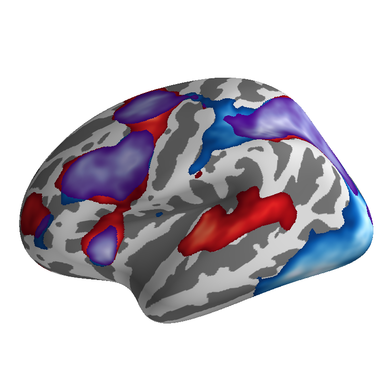
# Combine the two
conj_img = Image.blend(img1, img2, .5)
# Et voilà!
plt.figure()
plt.imshow(np.asarray(conj_img))
plt.show()
Cheers,
Michael