Hi,
I’m having issues obtaining topographic maps that look anything like what’s normally seen in the literature. See images. Basically, the maps are inconsistent and not reflecting what should be expected at the individual level, or the group level.
I suspect that my preprocessing may be wrong or incomplete, but it may be something else.
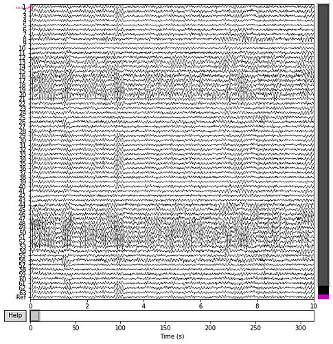
The files are individual subjects from Matlab. I’ve done preprocessing in a similar manner as Artoni & Michel (2025) How does Independent Component Analysis Preprocessing Affect EEG Microstates? with an additional 60-120Hz notch filter (see code below) and a different ICA method. I’ve included a screenshot of the psd and the full time scale of the channels in the post (please disregard channel 64 named ref). The full time scale of EEG looks a little rough but because the time period is large, it’s hard to tell. There are no artefacts, some drift at the end to the time segment. The psd looks fine and the filters seem to be doing their job.
I’m getting plenty of GFP peaks and the segmentation seems to be working. Until i get satisfying topographic maps, i’m not sure i should interpret any statistical test or even the quality of the segmentation.
I’ve tried many different n_cluster settings in ModKMeans(), different min_peak_distance settings in extract_gfp_peaks(). I’ve tried resampling from GFP or epochs but nothing changed.
See images and preprocessing code below.
GFP peaks:
Out[152]: < ChData | 12480 samples >
Thanks in advance for any help.
EEG:
- Brain Products ActiCap/ActiChamp
- montage: 64 Channels (+3 EOG); easycap-M43
- Length of recording: 310secs (size77501)
Software:
- Pycrostates 0.6.1
- Spyder version: 5.4.5 (conda)
- Python version: 3.11.5 64-bit
- Qt version: 5.15.8
- PyQt5 version: 5.15.9
- Operating System: macOS-14.6.1-x86_64-i386-64bit
# Preprocessing step largely inspired by Artoni & Michel (2025) *How does Independent Component Analysis Preprocessing Affect EEG Microstates?*
import os
import numpy as np
import sys
import subprocess
import matplotlib
from pycrostates.preprocessing import extract_gfp_peaks, apply_spatial_filter, resample
from pycrostates.cluster import ModKMeans
from scipy.signal import cheby2, filtfilt
import scipy.io as sio
from scipy.stats import kurtosis
import mne
from mne_icalabel import label_components
from mne.channels import find_ch_adjacency
from mne.viz import plot_ch_adjacency, plot_topomap


# Verbose mne
mne.set_log_level('info')

# --- Load Groups from a Matlab File ---
x_file = "~/[...].mat" # <--- --- --- --- --- --- --- --- --- ---
x_data = sio.loadmat(x_file)
x_scores = x_data["x"].flatten()
HS = np.where(x_scores > 8)[0] + 1
LS = np.where(x_scores < 4)[0] + 1
MS = np.setdiff1d(np.arange(1, len(x_scores) + 1), np.concatenate((HS, LS)))

# --- Load Standard EasyCap Montage ---
montage = mne.channels.make_standard_montage("easycap-M43")

data_path = "/[...]folder_x" # <--- --- --- --- --- --- --- --- --- ---
sfreq = 250

# Storage structures
subject_data = {}  # Store individual subject data
group_data = {"HS": [], "LS": [], "MS": []}  # Store group-level data
all_data = {}  # Store everything

save_dir = "/[...]folder_x" # <--- --- --- --- --- --- --- --- --- ---
os.makedirs(save_dir, exist_ok=True)

for idx in range(len(x_scores)):
    subject_id = idx + 1
    file_name = os.path.join(data_path, f"S_{subject_id}_epoched_data.mat") # <--- --- --- --- --- --- --- --- --- ---

    if os.path.exists(file_name):
        mat_data = sio.loadmat(file_name)

        if "F" in mat_data:
            eeg_data = mat_data["F"]

            num_channels = eeg_data.shape[0]

            # Channel ID
            raw_channel_names = montage.ch_names[:64] + ["EOG1", "EOG2", "EOG3"]
            ch_types = ["eeg"] * 64 + ["eog"] * 3
            info = mne.create_info(ch_names=raw_channel_names, sfreq=sfreq, ch_types=ch_types)
            raw = mne.io.RawArray(eeg_data, info)
            raw.set_montage(montage, on_missing="ignore")

            # --- Preprocessing ---
            # Chebyshev type II filters
            raw.filter(l_freq=1, h_freq=None, method='iir', iir_params=dict(order=24, ftype='cheby2', rs=25))
            raw.filter(l_freq=None, h_freq=45, method='iir', iir_params=dict(order=70, ftype='cheby2', rs=30))
            raw.notch_filter(freqs=[60, 120], method="fir")
            # 250Hz check
            if raw.info['sfreq'] != 250:
                raw.resample(250)

            def detect_bad_channels_kurtosis(raw, threshold=6): # Kurtosis threshold from Artoni & Michel 2025
                data = raw.get_data(picks="eeg")  # Pick only EEG channels (exclude EOG)
                kurt_vals = kurtosis(data, axis=1, fisher=False)  # Compute kurtosis for each channel
                # Use IQR method for robust thresholding
                Q1, Q3 = np.percentile(kurt_vals, [25, 75])
                iqr = Q3 - Q1
                upper_bound = Q3 + (threshold * iqr)
                bad_channels = [raw.ch_names[i] for i in range(len(kurt_vals)) if kurt_vals[i] > upper_bound]

                return bad_channels

            # Detect bad channels and update info
            bad_channels = detect_bad_channels_kurtosis(raw)
            raw.info['bads'] = bad_channels
            # Interpolating bad channels using Splines
            if raw.info['bads']:
                print(f"---------- ----------> Identified bad channels: {bad_channels} <---------- ---------- ")
                raw.interpolate_bads()
            else:
                print(f"\nNo bad channels detected. Skipping interpolation.\n")

            # Reference to average
            raw.set_eeg_reference("average")

            # --- Picard ICA --- (Converges better than fastICA)
            ica = mne.preprocessing.ICA(n_components=40, max_iter=2000, method='picard', random_state=42)

            # Run ICA on cleaned data
            ica.fit(raw)

            # Detect EOG-related artifacts using the 3 EOG channels AFTER fitting ICA
            eog_indices, eog_scores = ica.find_bads_eog(raw, ch_name=["EOG1", "EOG2", "EOG3"])

            # Apply a temporary 1-100 Hz filter for ICLabel classification (Error pop up even though there is a 1-100Hz filter)
            raw_for_iclabel = raw.copy()
            raw_for_iclabel.filter(l_freq=1.0, h_freq=100.0, method="iir", iir_params=dict(order=8, ftype='cheby2', rs=30))

            # Run ICLabel
            ic_labels = label_components(raw_for_iclabel, ica, method="iclabel")
            labels = ic_labels["labels"]
            scores = ic_labels["y_pred_proba"]

            # Identify and exclude high-confidence artifacts
            artifact_indices = [
                i for i, label in enumerate(labels)
                if label in ["muscle", "heart", "line_noise", "channel_noise", "other"]
                and scores[i] > 0.80]
            # Print detected artifacts
            if artifact_indices:
                print(f"Detected Artifacts:")
                for i in artifact_indices:
                    print(f"   - Component {i}: {labels[i]} (Confidence: {scores[i]:.2f})")
            else:
                print(f"No Artifacts Detected")

            # Combine artefacts with EOG components
            ica.exclude = list(set(eog_indices + artifact_indices))

            # Apply ICA correction
            raw = ica.apply(raw)

            # --- Apply Spatial Filtering to Enhance Microstates at the individual level
            raw = apply_spatial_filter(raw, exclude_bads=True)

            subject_data[subject_id] = {
                "raw": raw,
                "bad_channels": bad_channels,
                "ICA_components": ica,
                "labels": ic_labels["labels"],}

            # Save raw data
            raw_save_path = os.path.join(save_dir, f"subject_{subject_id}_raw.fif") <--- --- --- ---
            raw.save(raw_save_path, overwrite=True)
            if subject_id in HS:
                group_data["HS"].append(subject_data[subject_id])
            elif subject_id in LS:
                group_data["LS"].append(subject_data[subject_id])
            else:
                group_data["MS"].append(subject_data[subject_id])
        else:
            print(f"Skipping {file_name}: 'F' key not found in .mat file.")
    else:
        print(f"Skipping {file_name}: File not found.")


