Unusual failure mode of ICA in particular subject

Hi all,

I’m having a weird issue with ICA on one of my subjects. Before I describe the problem, I want to make it clear that this exact code works fine for all of my subjects except this one. Usually, ICA results in 80 sensible components (usually two cardiac components and a number of blink/MOG components). I identify these artefactual components manually and project them out using ica.exclude and ica.apply. It generally works very well to remove blink and heartbeat artifacts (they are no longer visible in the filtered data in the raw or PSD plots).

The issue happens with a particular resting-state recording (CTF-275, 1200 Hz sampling rate, 5 minutes) from the open dataset I am looking at (Mother Of all Unification Studies, available on Donders repo.)

I first load the MEG file, broadband filter, and apply reference array gradiometry:

filepath = op.join(megpath, restdatapath)
raw = mne.io.read_raw(filepath, preload=False)  # read raw data, don't load yet
raw.pick_types(meg=True, eeg=False) # get rid of EEG channels

filtered = raw.copy()
filtered.load_data()
filtered.filter(l_freq=1.0, h_freq=150.)  # FIR filter from 0.1-150 Hz

filtered.apply_gradient_compensation(grade=3) # apply gradiometry
filtered_orig = filtered.copy()  # make another copy for post-ICA comparison

Then do ICA with 80 components:

ica = mne.preprocessing.ICA(n_components=80, random_state=40, 
    method='picard', max_iter=1500)

ica.fit(filtered, decim=4)  # 1200/4 = 300 Hz = 150 * 2 (Nyquist limit)

which outputs the following:

# Subject has no previous ICA.  Computing...
# Fitting ICA to data using 273 channels (please be patient, this may take a while)
# Removing 5 compensators from info because not all compensation channels were picked.
# Selecting by number: 80 components
# Fitting ICA took 48.0s.

Here is a plot of the first 10 components and their respective time courses:

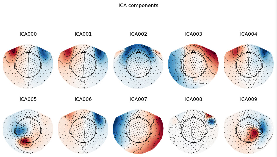
Looks relatively sensible so far. One thing I noticed about this recording in particular is that the ICA seems to pull out two EOG components (ICA000, ICA001) with very similar topography. This is stable across the different ICA implementations (infomax, picard, fastica etc.) and with different parameters (within reason). The issue occurs when I try to project out one or both of these components. I will project out ICA000 just to demonstrate:

ica.exclude=[0]
ica.apply(filtered)

This reports:

#    Applying ICA to Raw instance
#    Transforming to ICA space (80 components)
#    Zeroing out 1 ICA component
#    Projecting back using 273 PCA components
#   <RawCTF | sub-A2011_task-rest_meg.meg4, 301 x 368298 (306.9 s), ~846.3 MB, data loaded>

If I then plot the PSD of the ICA-applied data next to the original, it becomes clear that something very bad has happened:

The ICA-applied data (upper plot) shows broadband noise which didn’t exist in the original (lower plot). Furthermore, this synthetic noise appears to have the topography of the ICA component we tried to project out:

Does anyone have any clue what’s happening here? Maybe some kind of numerical instability in the algorithm? Or perhaps I am being silly.

Here is my platform information: I’m using MNE version 0.22 (stable) running inside WSL2 in Windows 10. I haven’t encountered any issues like this before with MNE – as I said, this just happens with the one subject (sub-A2011 in the MOUS dataset – it’s open to download, you have to sign up to an eduID account). In all other subjects the ICA works properly, eye blinks and heartbeats are cleaned, and I can proceed with analysis.

I’d be grateful if anyone has any ideas or pointers. Thanks for reading!

Platform:      Linux-5.4.72-microsoft-standard-WSL2-x86_64-with-glibc2.10
Python:        3.8.8 | packaged by conda-forge | (default, Feb 20 2021, 16:22:27)  [GCC 9.3.0]
Executable:    /home/neurons/miniconda3/envs/mne-sktime/bin/python
CPU:           x86_64: 12 cores
Memory:        25.0 GB

mne:           0.22.0
numpy:         1.20.2 {blas=NO_ATLAS_INFO, lapack=lapack}
scipy:         1.6.2
matplotlib:    3.3.4 {backend=Qt5Agg}

sklearn:       0.24.1
numba:         0.51.2
nibabel:       3.2.1
nilearn:       0.7.1
dipy:          1.4.0
cupy:          Not found
pandas:        1.2.3
mayavi:        4.7.2
pyvista:       0.29.0 {pyvistaqt=0.3.0, OpenGL 3.3 (Core Profile) Mesa 20.0.8 via llvmpipe (LLVM 10.0.0, 128 bits)}
vtk:           9.0.1
PyQt5:         5.12.3

I don’t know what’s going on but just to let you know I can replicate on this same file.

Maybe I’ll find some time tomorrow to investigate.

let me know if you understand anything. Using less components or removing the ref_meg channels did not help.
Neither did help to set the n_pca_components parameter in apply method.

Alex

1 Like

Thank you for taking the time to replicate the issue. I will certainly post in this thread if I discover anything new.

Gill

Hi Gill,

I quickly discussed this issue with Jan-Mathijs Schoffelen (who is also the author of the MOUS data).

We came to the following conclusions:
It seems that the component not only captures the eye movement of interest, but also some non-specific residual high-frequency noise. If you then remove the weighted ICA component from each of the sensors, this noise can be “added” in. This effect could be further enhanced in your case by the downsampling of the data you fit the ICA on, but not when removing the component(s) - the fitted components “know” less about the high frequency activity because you have removed some of it from the data you fit your ICA on.

Have you tried also removing the components 1, 2, 4, and 6 in addition to component 0? Especially component 4 seems to specifically capture the high frequency noise associated with the frontal channels in this recording.

Britta

Hello Britta,

Thank you very much for looking at this. I tried your suggestion and it worked! Here is the effect with components 0, 1, 2, 4, 6 removed:

I think it was the absence of component 4 causing the problem. The high frequency noise in component 0 must be almost exactly anti-correlated with the noise in component 4. I don’t really understand how this happens in the first place!

I’m not sure the downsampling was affecting anything: I made sure to filter the data between 1-150 Hz as a first step, and then downsampling to 300 Hz ensures that the Nyquist criterion is met. I tried again without downsampling (fs = 1200 Hz) and had the same issue.

It’s very strange that I’ve only encountered this problem once in 40 subjects. I’m looking into identifying artefact components in an automated way and this might be a non-trivial edge case. Do you think it might be sensible to use e.g. corrmap to detect components with very similar topography and tag those as bad too? The problem is that there are cases when it seems to have worked properly but you can still see the spatial signature of the blinks in the 50-100 Hz region. It’s difficult to know which combination of components is “correct”. Do you have any idea how to avoid this problem in the future?

Thanks again,

Gill

1 Like

Hi Gill,

I am glad this worked!
Regarding your question as to why this happened: you can see in your first plot, that all these components have distinct time series (despite similar topographies), so I assume this is why they were classified as independent components by the ICA algorithm.

I do not have much experience with automated ICA processing, but assume that corrmap could work, I think there is even an example on something similar on the MNE homepage; if I remember correctly. Probably not crucial for this artifact and its topography but possibly others: you would need to make sure not to throw out genuine activity with automated processing - the problem goes both ways I guess.

Good luck trying it out!
Britta

2 Likes

So, months later I returned to this problem, and eventually found that increasing the highpass filter value from 1 Hz to 4 Hz fixes things. The guidelines for using ICA mention that the data has to be free of low-frequency drifts in order for the algorithm to work properly, and I think the low-frequency drifts in this dataset were simply stronger than in others, which results in the low frequencies leaking through the filter. I ran into the issue in some other datasets with strong low-frequency drifts, and it worked on those too. I imagine using a steeper roll-off might also achieve the same thing, though I don’t want to mess with the default filter settings.

I hope this helps if someone has the same issue!

1 Like